Analysis of Consumer Behaviors in Pandemic

Introduction

This part analyze the changes to consumer behaviors during the pandemic based on national consumption expenditure data retrieved from Bureau of Economic Analysis (BEA).

Will we ever spend our money like the good old days?  

Consumption and Covid

joint_plot = plot_ly(covid_consumption, x = ~time) %>% 
  add_trace(y = ~consumption, type = "scatter", mode = "lines", color = ~functions, yaixs = "y") %>% 
  add_trace(y = ~quarterly, type = "bar", name = "Covid Cases", yaxis = "y2", opacity = 0.6, marker = list(color = 'rgb(158,202,225)'))  %>% 
  layout(title = "Consumption of Goods and Services Compared with Covid Cases",
         yaxis=list(title = "consumption expenditure", side="left"),
         yaxis2=list(title = "covid cases", side="right", overlaying="y"),
         showlegend=TRUE)

joint_plot

The lowest point actually did not happen as expected at the peak of the pandemic but at the second quarter of 2020, when cases just start to rise.

Consumption expenditures of services experienced a steeper change than expenditures of goods due to the shutdown of businesses, the quarantine and the lock down policies etc.

Even though cases keep rising, as restrictions keep lifting, the rate of vaccination keep rising, economics keep recovering, people’s consumption expenditure grows steadly after the third quarter of 2020.

The total consumption expenditure is even larger by now comparing with that before the pandemic. This can be partially explained by inflation and government’s stimulus plan.

 

Consumption of Goods

general_2 = consumption_function %>% 
  filter(functions %in% c("Durable goods","Nondurable goods","household","nonprofit consumption")) %>% 
  select(-line) %>% 
  pivot_wider(names_from = functions, values_from = consumption) %>% 
  janitor::clean_names()

subfig_1 = plot_ly(general_2, x = ~time, y = ~durable_goods, type = "bar", name = "Durable Goods", marker = list(color = 'rgb(49,130,189)')) %>% 
  add_trace(y = ~nondurable_goods, name = "Nondurable Goods", marker = list(color = 'rgb(204,204,204)')) %>% 
  layout(title = "Decomposition of Consumption of Goods",
         yaxis = list(title = "Consumption"), barmode = "stack",
         legend = list(orientation = 'h', x = 0, y = -0.2))

subfig_1

The proportion of the nondurable goods such as food, drinks and clothing etc. increased after the second quarter of 2020, the time when the cases are rising. People are more willing to spend income on the nonduarble goods instead of spending them on buying the durable goods such as cars and house.

There is a lowest point of the value of consumption expenditure in all kind of goods consumption in the second quarter of 2020, when the COVID-19 outbroke, and after that, the consumption gradually grow up.

Durable Goods

durable_goods = 
  consumption_function %>% 
  filter(functions %in% c("Motor vehicles and parts","Furnishings and durable household equipment","Recreational goods and vehicles","Other durable goods")) 

durable_goods %>% 
  plot_ly(x = ~time, y = ~consumption, type = 'scatter', mode = 'lines', yaxis="y", line = list(simplyfy = F), color = ~functions) %>% 
  layout(title = "Decomposition of Consumption in Durable Goods", 
    legend = list(orientation = 'h', x = 0, y = -0.2)) 

Motor vehicles and parts increases fastest after experiencing the bottom point, from which we can infer that people go out even more frequently after the pandemic than before the pandemic.

Recrational goods and vehicles(includes video/audio equipments and sporting equipments) keep increasing during the pandemic because people are spending more time at home instead of socializing.

Furnishngs and durable household equipment consumption value barely reduced in the pandemic, and there is a growth after the second quarter of 2020 probably because people’s demand on durable goods like this does not change significantly due to the pandemic, on the contrary, staying at home increases people’s willingness to buy furniture.

Other durable goods includes jewelry and watches, therapeutic appliances, educational books, luggages, and telephones and related. Like most of other kinds of products, the value of expenditure experienced a lowest point at the second quarter of 2020 and recovered after that.

Nondurable Goods

The proportion of consumption expenditure on food/beverages and other nondurable goods exceeds a lot than that of clothing/footware and energy goods. Unlike the changes in consumption of clothing/footware and energy goods, that in food/beverages and other nondurable goods is not experiencing reduction in the pandemic but increases steadly.

nondurable_goods = 
  consumption_function %>% 
  filter(functions %in% c("Food and beverages purchased for off-premises consumption","Clothing and footwear","Gasoline and other energy goods","Other nondurable goods")) 

nondurable_goods %>% 
  plot_ly(x = ~time, y = ~consumption, type = 'scatter', mode = 'lines', yaxis="y", color = ~functions) %>% 
  layout(title = "Decompostion of Consumption in Nondurable Goods",
         legend = list(orientation = 'h', x = 0, y = -0.2))

Clothing and footwear consumption reduces rapidly in the pandemic because people began to work from home, and didn’t need to go outside to socialize.

Similar to changes in motor vehicles, the consumption expenditure in Gasoline and other energy goods experienced significant decline in the second quarter of 2020 due to reductions in transportation. Consumption in energy goods by the end of 2021 has already surpassed that in 2019 probably due to increase in gasoline prices in the United States.

The small peak in the second quarter in 2020 in the consumption of food and beverages results from people spending more time at home and reduced the frequency of dining outside.

Other nondurable goods includes medical products, recreational items, household supplies, personal care products, tobacco, and magazines/newspapers. Similar to that of food and beverages, the total consumption of this category keep increasing and exceeds the value before the pandemic.

 

Consumption of Services

The consumption of services is calculated with two categories: household consumption expenditures for services, and final consumption expenditures of nonprofit institutions serving households (nonprofit consumption). We can see the consumption value of nonprofit institutions remain steady comparing with household services from 2019 till now.

Since we are focusing on consumer behavior analysis in our project, we only analyze the part of household consumption expenditures of services.

subfig_2 = plot_ly(general_2, x = ~time, y = ~household, type = "bar", name = "Household", marker = list(color = 'rgb(49,130,189)')) %>% 
  add_trace(y = ~nonprofit_consumption, name = "Nonprofit Consumption", marker = list(color = 'rgb(204,204,204)')) %>% 
  layout(title = "Decomposition of Consumption in Services ",
         yaxis = list(title = "Consumption"), barmode = "stack",
         legend = list(orientation = 'h', x = 0, y = -0.2))

subfig_2

Household Services

Except for housing and utilities and finantial service and insurance, the consumption expenditure of all kinds of household services experienced a sharp decline in the second quarter of 2020.

household_consumption =
  consumption_function %>% 
  filter(functions %in% c("Housing and utilities","Health care","Transportation services","Recreation services","Food services and accommodations","Financial services and insurance","Other services")) 

household_consumption %>% 
  plot_ly(x = ~time, y = ~consumption, type = 'scatter', mode = 'lines', yaxis="y", color = ~functions) %>% 
  layout(title = "Decomposition of Consumption in Household Services",
         legend = list(orientation = 'h', x = 0, y = -0.2))

Consumption of Health care reduced significantly in the second quarter of 2020 because the hospital didn’t have enough ability to take in other patients due to increasing cases of Covid.

Transpotation service includes motor vehicle services and public transportation. The total consumption of transportation hasn’t recovered to the level before the pandemic by the third quarter of 2021.

Food service and accommodations reduced because most of the restaurants were shut down in the pandemic. By the third quarter of 2021, the value in this category reached to a new highest level due to increase in price and the recovery of dining services.

Recreation service mainly consists of the fees of the activities for fun such as sport, museum, gambling, package tour etc. The value of consumption reduced significantly in the second quarter of 2020 due to social-distancing.

Different to other consumption categories, housing and utilities(which mainly includes housing rental and the fees for the resources at home such as electricity and gas) and financial service and insurance (which mainly includes life and health insurance and commissions in banks) increased.

 

Engel Coefficient

“The poorer is a family, the greater is the proportion of the total outgo [family expenditures] which must be used for food. …The proportion of the outgo used for food, other things being equal is the best measure of the material standard of living of a population.”

The following chart displays the changing trend in Engel Coefficient ever since Covid-19 outbreak.

total = consumption_product %>% 
  filter(products == "Personal consumption expenditures")

engel = nondurable_goods %>% 
  filter(functions == "Food and beverages purchased for off-premises consumption") %>% 
  left_join(total, by = 'time') %>% 
  select(time, consumption.x, consumption.y)

colnames(engel) = c("time", "food", "total")

engel = engel %>% 
  mutate(engel_coef = as.numeric(food)/as.numeric(total))

plot_ly(engel, x = ~time, y = ~engel_coef, type = 'scatter', mode = 'lines') %>% 
  layout(title = "Changes in Engel Coefficient",
         yaxis = list(title = "Engel Coefficient"))

From the changing trend we can see: although the engel coefficient has dropped from the highest level when the pandemic started, we are still at a much higher level compared with that before the pandemic.

 

Consumption Structure Analysis

This part visualizes the the percentage of the consumption expenditures of different categories of products in durable goods, nondurable goods, and services.

By the comparison between first quarter in 2019, second quarter in 2020, third quarter in 2021, percentages changed in the second quarter of 2020, but there is no significant changes observed in proportion of different categories of consumption before the consumption and now.

This is good news (in some ways)! At least we are returning back to normal…
But still be careful with the Omicron!

Durable Goods

Recreational goods and vehicles increased its proportion to the largest in the second quarter of 2020 and now returned to the level before the pandemic.

areas <- c(rgb(1, 0, 0, 0.25),
           rgb(0, 1, 0, 0.25),
           rgb(0, 0, 1, 0.25))

percent <- function(x) {
  if(is.numeric(x)){ 
    ifelse(is.na(x), x, paste0(round(x*100L, 2), "%")) 
  } else x 
}

durable_goods_radar = durable_goods %>% 
  filter(time %in% c("2019_q1", "2020_q2", "2021_q3")) %>% 
  select(functions, time, consumption)  %>% 
  pivot_wider(names_from = functions, values_from = consumption) 

total = rep(1,5)
start = rep(0,5)
durable_goods_radar = rbind(total, start, durable_goods_radar)[,-1]
rownames(durable_goods_radar) = c("1", "2", "2019_q1", "2020_q2","2021_q3")
colnames(durable_goods_radar) = c("motor", "furnishing", "recreation", "other")
durable_goods_radar[3,] = durable_goods_radar[3,]/1473292
durable_goods_radar[4,] = durable_goods_radar[4,]/1468253
durable_goods_radar[5,] = durable_goods_radar[5,]/1984391

durable_goods_radar[-c(1,2),] %>% 
  set_rownames(.,c("2019_q1", "2020_q2","2021_q3")) %>% 
  mutate_each(funs(percent)) %>% 
  knitr::kable()

	motor	furnishing	recreation	other
2019_q1	33.94%	23.88%	27.61%	14.57%
2020_q2	33.05%	24.6%	31.19%	11.16%
2021_q3	33.04%	23.66%	28.9%	14.4%

radar_1 = radarchart(durable_goods_radar,
                     cglty = 2, cglcol = "gray", pcol = 2:4, plwd = 1, plty = 2, seg = 2) 
legend("topright",
       legend = c("2019_q1", "2020_q2","2021_q3"),
       bty = "n", col = areas, pch = 20,
       text.col = "grey25", pt.cex = 2)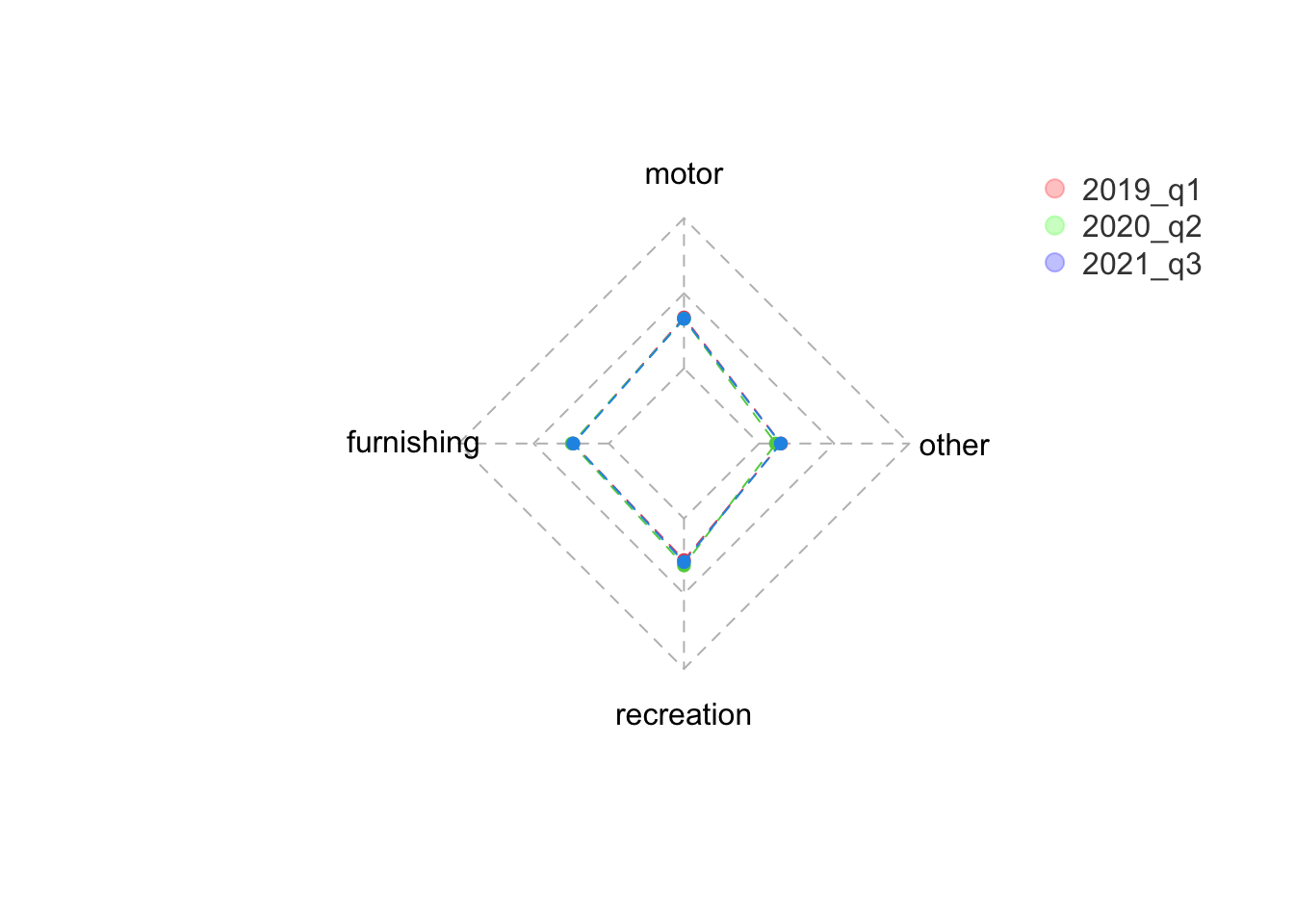

Nondurable Goods

The proportion of consumption in clothing and energy goods dropped significantly in the second quarter of 2020 while people spend more of their savings on food and beverages.

nondurable_goods_radar = nondurable_goods %>% 
  filter(time %in% c("2019_q1", "2020_q2", "2021_q3")) %>% 
  select(functions, time, consumption)  %>% 
  pivot_wider(names_from = functions, values_from = consumption) 

nondurable_goods_radar = rbind(total, start, nondurable_goods_radar)[,-1]
rownames(nondurable_goods_radar) = c("1", "2", "2019_q1", "2020_q2", "2021_q3")
colnames(nondurable_goods_radar) = c("food/beverage", "clothing", "energy", "other")
nondurable_goods_radar[3,] = nondurable_goods_radar[3,]/2909515
nondurable_goods_radar[4,] = nondurable_goods_radar[4,]/2881659
nondurable_goods_radar[5,] = nondurable_goods_radar[5,]/3509766

nondurable_goods_radar[-c(1,2),] %>% 
  set_rownames(.,c("2019_q1", "2020_q2","2021_q3")) %>% 
  mutate_each(funs(percent)) %>% 
  knitr::kable()

	food/beverage	clothing	energy	other
2019_q1	34.83%	13.52%	11.13%	40.52%
2020_q2	39.98%	10.19%	6.54%	43.29%
2021_q3	35.51%	13.68%	10.78%	40.03%

radar_2 = radarchart(nondurable_goods_radar,
                     cglty = 2, cglcol = "gray", pcol = 2:4, plwd = 1, plty = 2, seg = 2)
legend("topright",
       legend = c("2019_q1", "2020_q2","2021_q3"),
       bty = "n", col = areas, pch = 20,
       text.col = "grey25", pt.cex = 2)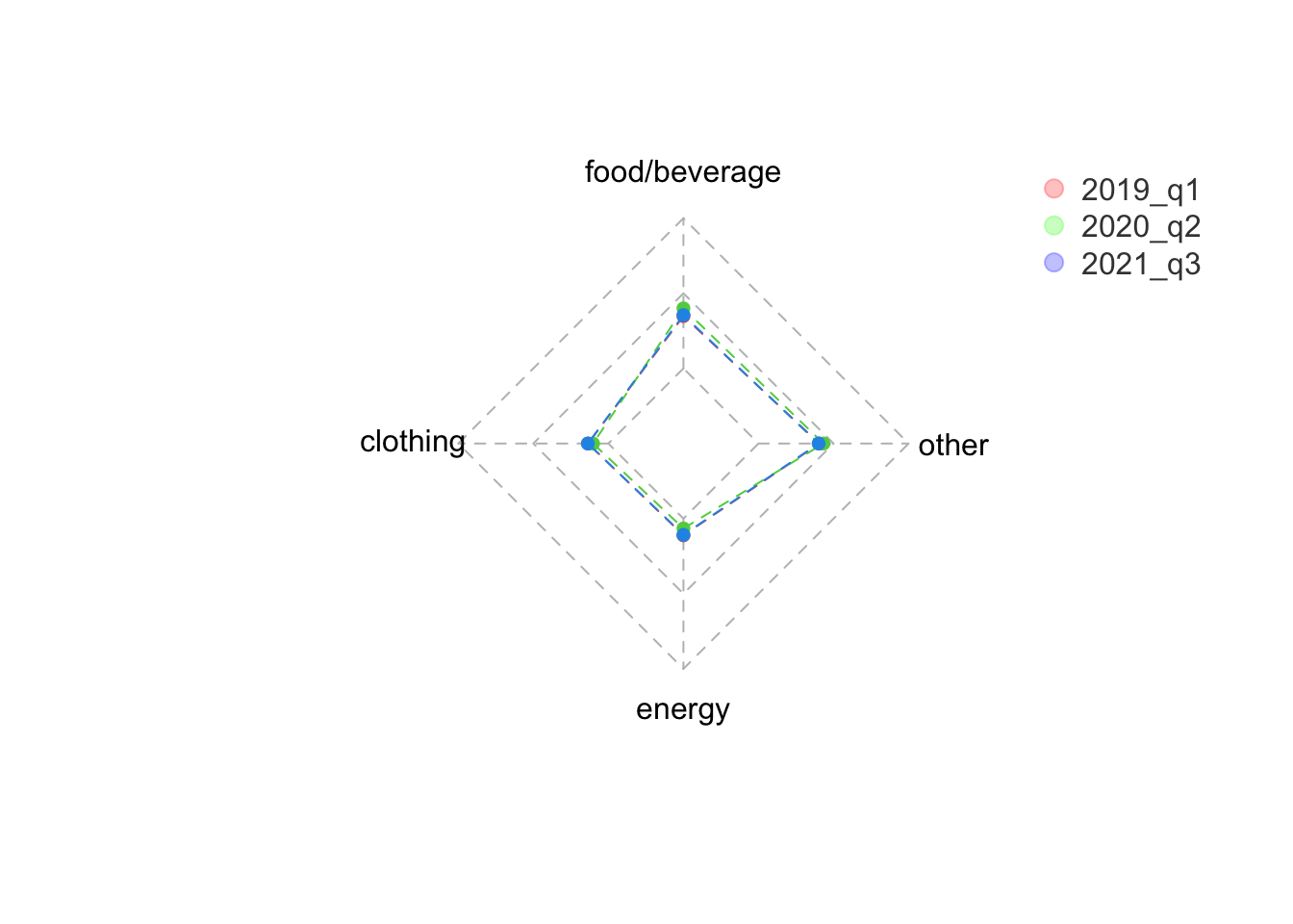

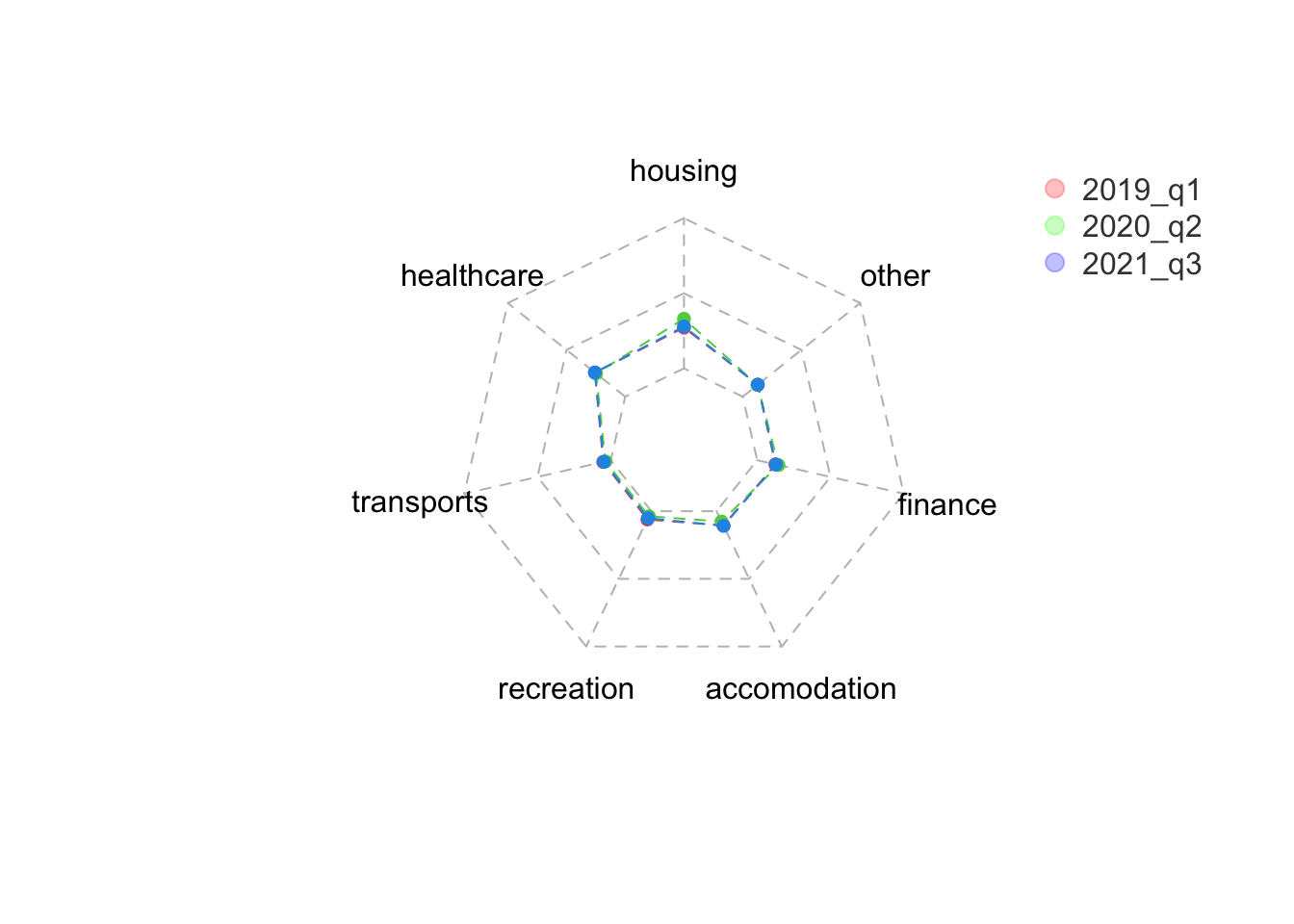
Household Services

The proportion of consumption on housing increased significantly, and the proportion spent on financial services increased a little while people spend less of their savings on the other categories of household services

household_consumption_radar = household_consumption %>% 
  filter(time %in% c("2019_q1", "2020_q2","2021_q3")) %>% 
  select(functions, time, consumption)  %>% 
  pivot_wider(names_from = functions, values_from = consumption) 

total = rep(1,8)
start = rep(0,8)
household_consumption_radar = rbind(total, start, household_consumption_radar)[,-1]
rownames(household_consumption_radar) = c("1", "2", "2019_q1", "2020_q2","2021_q3")
colnames(household_consumption_radar) = c("housing", "healthcare", "transports", "recreation", "accomodation", "finance", "other")
household_consumption_radar[3,] = household_consumption_radar[3,]/9336650
household_consumption_radar[4,] = household_consumption_radar[4,]/8062770
household_consumption_radar[5,] = household_consumption_radar[5,]/9984527

household_consumption_radar[-c(1,2),] %>% 
  set_rownames(.,c("2019_q1", "2020_q2","2021_q3")) %>% 
  mutate_each(funs(percent)) %>% 
  knitr::kable()

	housing	healthcare	transports	recreation	accomodation	finance	other
2019_q1	27.15%	25.8%	5.14%	6.14%	10.57%	12.38%	12.82%
2020_q2	33.09%	24.81%	3.61%	3.77%	7.65%	14.5%	12.58%
2021_q3	27.93%	25.84%	4.62%	5.16%	10.84%	12.79%	12.82%

radar_3 = radarchart(household_consumption_radar,
                     cglty = 2, cglcol = "gray", pcol = 2:4, plwd = 1, plty = 2, seg = 2)
legend("topright",
       legend = c("2019_q1", "2020_q2","2021_q3"),
       bty = "n", col = areas, pch = 20,
       text.col = "grey25", pt.cex = 2)