Regression Model for Comsumption Prediction
COVID-19 pandemic has induced many economical problems. From the BEA published dataset in year 2021, we know that the personal income decreased $216.2 billion, or 1.0 percent at a monthly rate, while consumer spending increased $93.4 billion, or 0.6 percent, in September. The decrease in personal income primarily reflected the winding down of pandemic-related assistance programs (BEA, https://www.bea.gov/data/income-saving/personal-income).
For this project, we are interested in exploring how the COVID-19 pandemic affected people’s personal consumption (PCE) patterns. We know that one’s consumption is associate with one’s income, so we will build a model for PCE expenditure using income data and we want to show that there is significant change in PCE during the pandemic that cannot be explained by the income model, which works in pre-pandemic periods.
Model: Predict PCE based on multiple sources of personal income
We are interested in exploring the how the changes in the following sources of personal income might affect PCE:
Wages and salaries: wages and salaries received from employersSupplements to wages and salaries: supplemental payments received from employersSocial Security: benefits include old-age, survivors, and disability insurance benefits that are distributed from the federal old-age and survivors insurance trust fund and the disability insurance trust fundMedicare: benefits include hospital and supplementary medical insurance benefits that are distributed from the federal hospital insurance trust fund and the supplementary medical insurance trust fundPersonal Current Taxes: total personal tax payment
PCE:
Personal consumption expenditures(on goods and services)
We want to look at data from 1967 Quarter 1 to 2020 Quarter 4:
format_function <- function(input) {
  str_c(str_split(input, 'q')[[1]][1], ' Quarter ', str_split(input, 'q')[[1]][2])
}

pce_4720 <- read_excel("data/pce_1947_2020.xlsx", sheet = 'T20100-Q',
                      range = 'A8:KM54') %>%
  janitor::clean_names() %>%
  select(x2, x1967q1:x2020q4) %>%
  drop_na() %>%
  # We only want to look at several variables:
  filter(
      x2 == 'Wages and salaries' |
      x2 == 'Supplements to wages and salaries' |
      x2 == 'Social security' |
      x2 == 'Medicare' |
      x2 == 'Less: Personal current taxes' |
      x2 == 'Personal consumption expenditures'
  ) %>%
  pivot_longer(
    x1967q1:x2020q4,
    names_to = 'time',
    names_prefix = 'x',
    values_to = 'millions_of_dollars'
  ) %>%
  rename(variable = x2) %>%
  mutate(
    variable = ifelse(variable == 'Less: Personal current taxes', 'Personal current taxes', variable)
  )
  #separate(time, c("year", "quarter"), "q") %>%

pce_4720_formatted <- pce_4720 %>%
  mutate(
    time = map(.x = time, format_function)
  )

head(pce_4720_formatted) %>% knitr::kable(caption = 'Example of the Data from BEA')| variable | time | millions_of_dollars |
|---|---|---|
| Wages and salaries | 1967 Quarter 1 | 418841 |
| Wages and salaries | 1967 Quarter 2 | 423604 |
| Wages and salaries | 1967 Quarter 3 | 432009 |
| Wages and salaries | 1967 Quarter 4 | 441583 |
| Wages and salaries | 1968 Quarter 1 | 454210 |
| Wages and salaries | 1968 Quarter 2 | 465923 |
Data Overview
Let’s take a brief look at the changes of incomes and PCE over time:
fig_1 <- pce_4720_formatted %>%
  plot_ly(x = ~time, y = ~millions_of_dollars, type = "scatter", mode = "lines", color = ~variable) %>%
  layout(title = "<b> Spaghetti Plot for Personal Income and Dispositions v.s. PCE <b>") %>%
  layout(yaxis = list(title = "<i> Millions of Dollars (M) <i>"), barmode = "stack",
         xaxis = list(title = "<i> Time <i>"),
         legend = list(title = list(text = '<b> Dispositions </b>'))) %>%
  layout(legend = list(orientation = 'h', x = 0, y = -0.2))
fig_1
For all categories, there is a exponentially increasing trend as time proceeds. Note that there is a drop for incomes and PCE at year 2020.
We can also look at the time v.s. logarithm dollars graph. Clearly, there is a increasing trend as time proceeded, and there is a drop for multiple source of incomes at year 2020.
fig_2 <- pce_4720_formatted %>%
  plot_ly(x = ~time, y = ~log(millions_of_dollars), type = "scatter", mode = "lines", color = ~variable) %>%
  layout(title = "<b> Spaghetti Plot for log(Personal Income and Dispositions) v.s. PCE </b>", yaxis = list(title = "<i> log(Dollars) <i>"), barmode = "stack",
         xaxis = list(title = "<i> Time <i>"),
         legend = list(title = list(text = '<i> Dispositions </i>'))) %>%
  layout(legend = list(orientation = 'h', x = 0, y = -0.2))

fig_2
Model fitting
We hypothesize that the personal consumption expenditure pattern has changed with respect to personal income for pre- v.s. in-pandemic periods.
To test this hypothesis, we will fit a linear model using data from year 1967-2018, the “pre-pandemic” period. We will then use this model to predict for PCE outcomes for a pre-pandemic year, 2019, and a in-pandemic year, 2020, respectively. Then we will compare if there is significant difference between the root mean square errors (RMSE) between the pre-pandemic and in-pandemic periods. If there is significant difference between them, we can conclude that there is enough evidence showing that the personal consumption expenditures patterns has changed during the pandemic.
Fit a MLR model using data from 1967 - 2018 (pre-COVID-19 pandemic)
pce_4718_by_dis <-
  pce_4720 %>%
  filter(!str_detect(time, '2019|2020')) %>%
  pivot_wider(
    names_from = variable,
    values_from = millions_of_dollars
  ) %>%
  janitor::clean_names()

test1 <- lm(personal_consumption_expenditures ~ wages_and_salaries + social_security + supplements_to_wages_and_salaries + personal_current_taxes + medicare, data = pce_4718_by_dis)

test1 %>% broom::tidy() %>% knitr::kable(digits = 3, caption = "MLR model PCE v.s. income sources")| term | estimate | std.error | statistic | p.value |
|---|---|---|---|---|
| (Intercept) | 21183.961 | 15610.049 | 1.357 | 0.176 |
| wages_and_salaries | 0.878 | 0.052 | 16.757 | 0.000 |
| social_security | -0.456 | 0.186 | -2.452 | 0.015 |
| supplements_to_wages_and_salaries | 1.966 | 0.172 | 11.449 | 0.000 |
| personal_current_taxes | -0.176 | 0.070 | -2.526 | 0.012 |
| medicare | 4.030 | 0.154 | 26.231 | 0.000 |
The adjusted \(R^2\) value for the MLR model is 0.9998252, meaning that the our model ‘fits’ the data well.
To further improve the model, we want to determine whether we should transform our variables for a better fit result or not. To check this, we will use Box-Cox transformation:
plot(test1)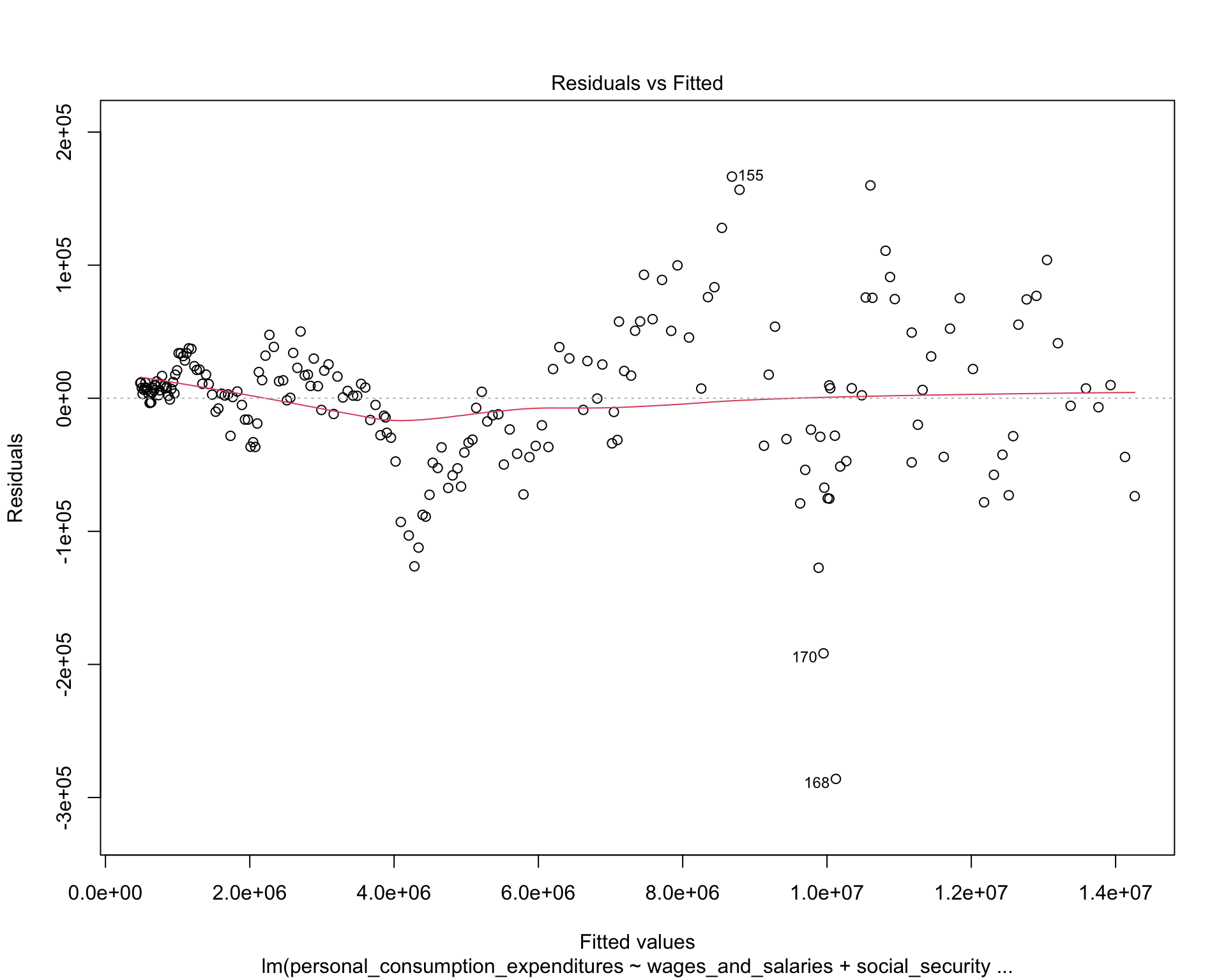
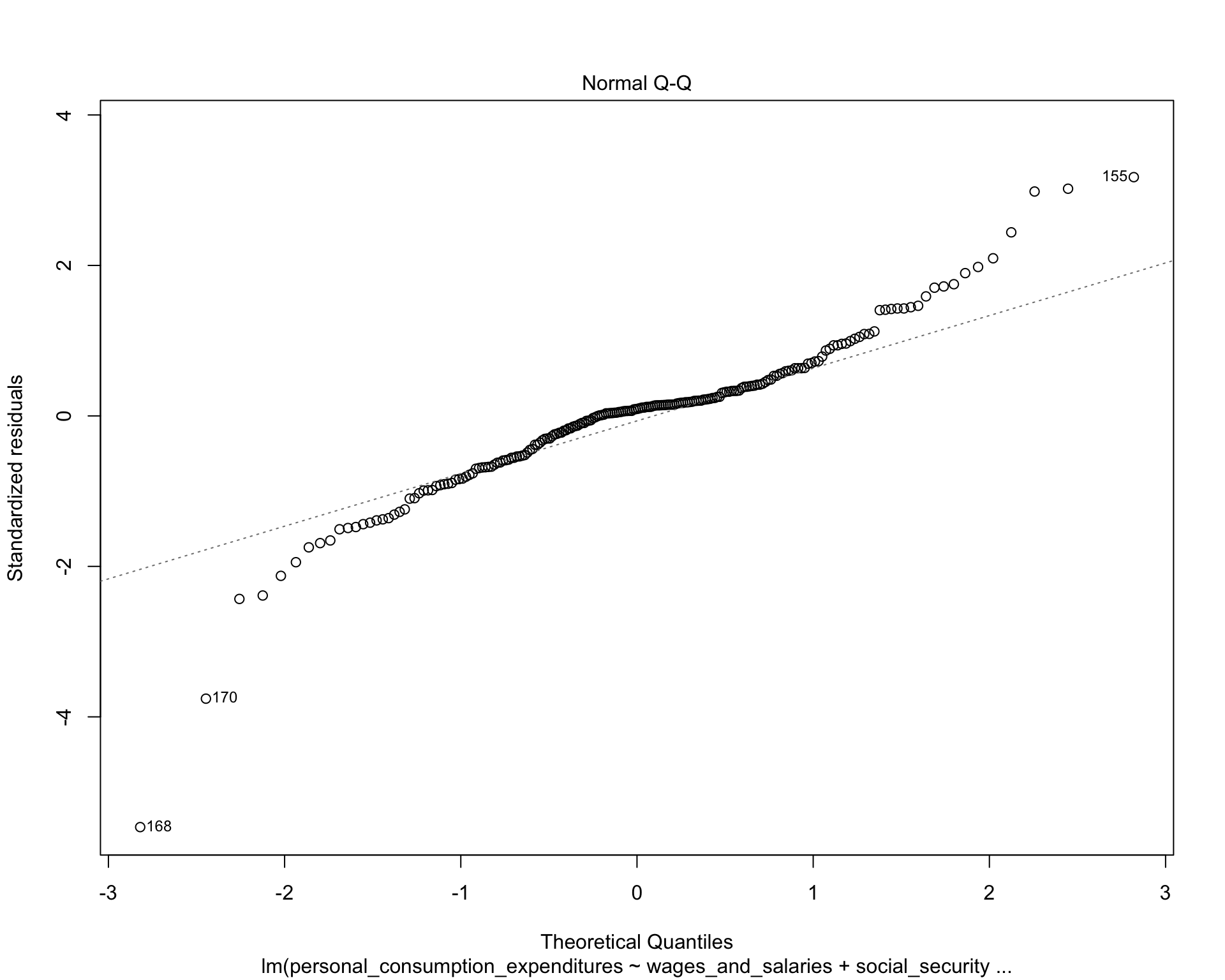
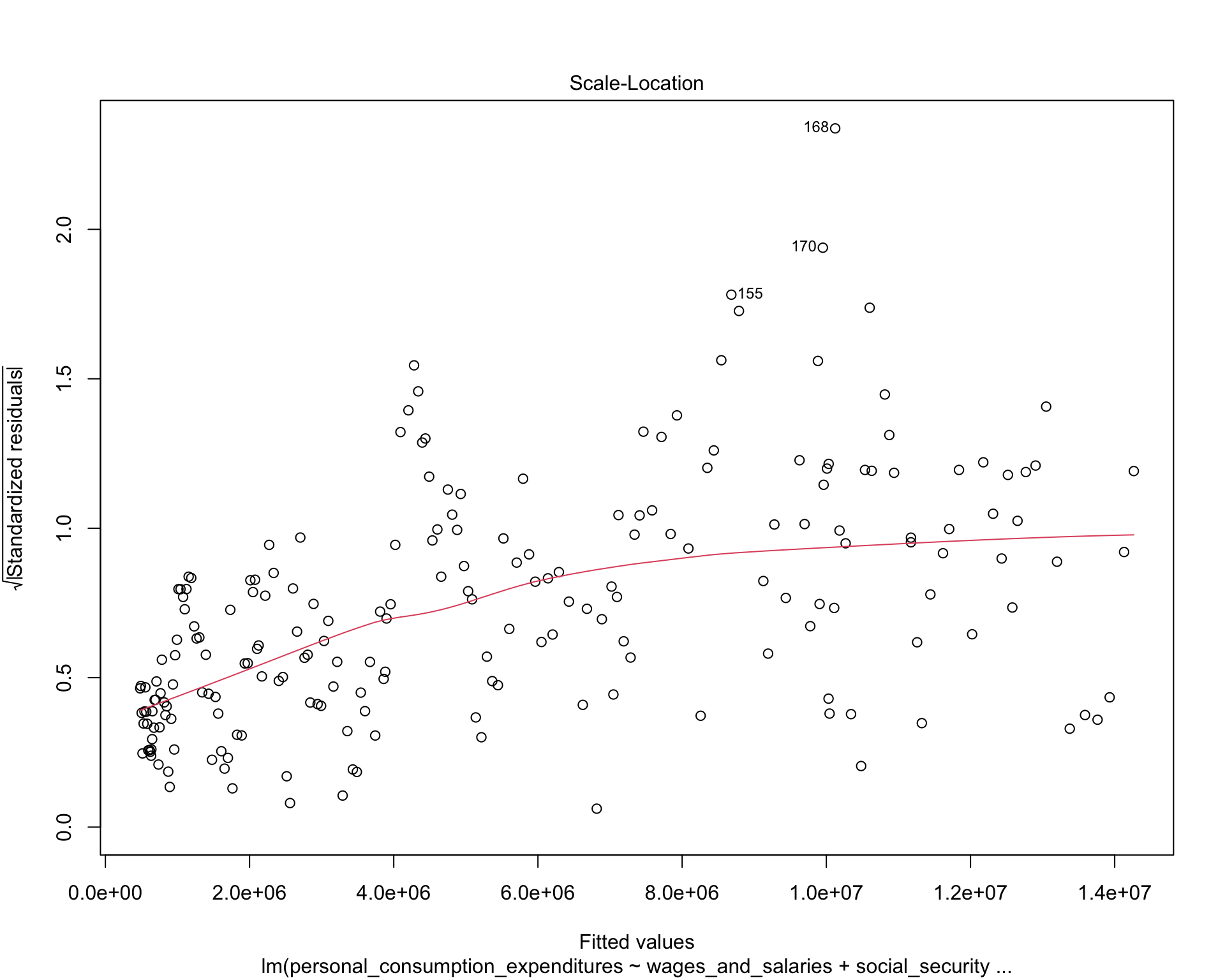
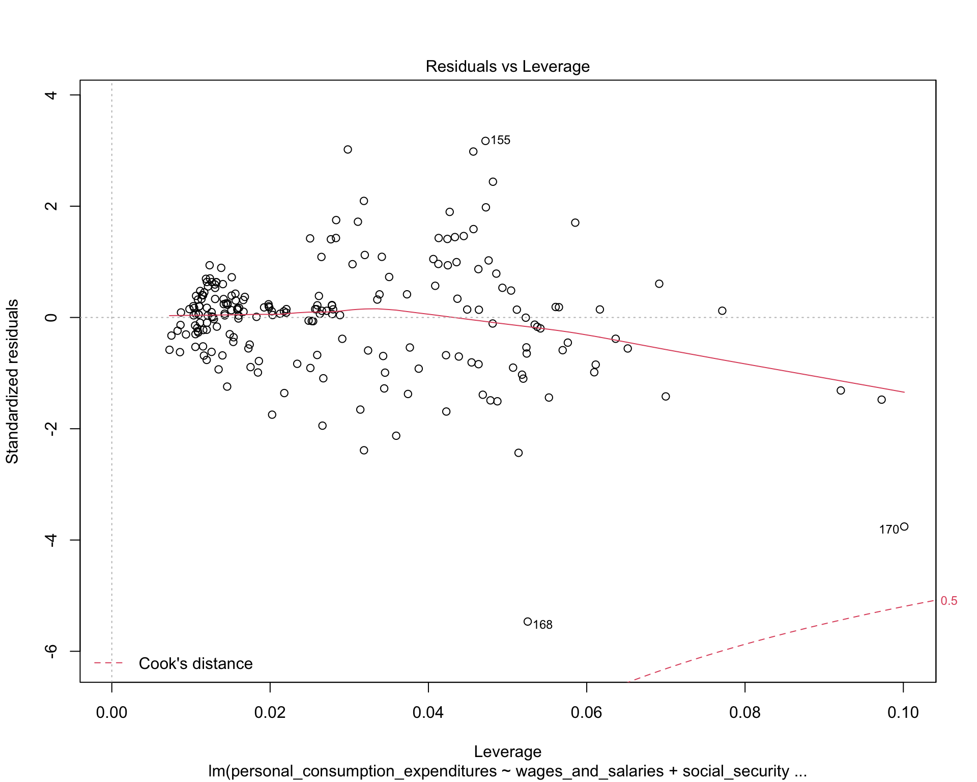
MASS::boxcox(test1)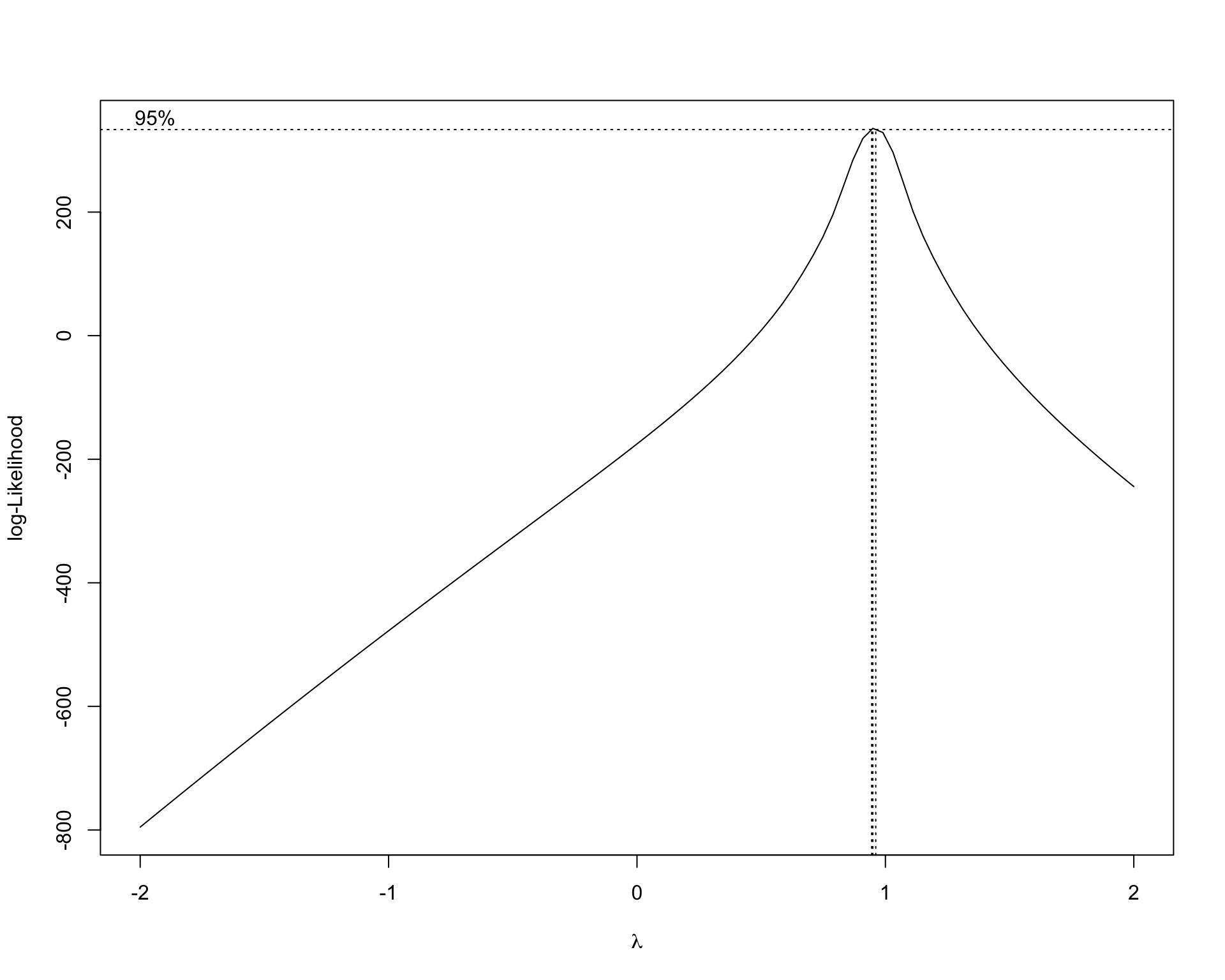
The QQ-plot indicates the distribution of residuals are normal. The Scale-location plot shows that the residuals are spread equally along the range of predictors. And the residuals-leverage plot shows that no outlier is influential.
Therefore, the relationships between income sources and PCE are best approximated by linear function. We can use MLR model in the following analysis.
Prediction
We will predict the PCE for year 2019 and year 2020 using our MLR model:
pce_2019 <-
  pce_4720 %>%
  filter(
    str_detect(time, '2019')
  ) %>%
  pivot_wider(
    names_from = variable,
    values_from = millions_of_dollars
  ) %>%
  janitor::clean_names()

pce_2019_pred <- predict(test1,pce_2019)

#RMSQ
rmse19 <- rmse(test1, pce_2019)

pce_2020 <-
  pce_4720 %>%
  filter(
    str_detect(time, '2020')
  ) %>%
  pivot_wider(
    names_from = variable,
    values_from = millions_of_dollars
  ) %>%
  janitor::clean_names()

pce_2020_pred <- predict(test1,pce_2020)

#RMSQ
rmse20 <- rmse(test1, pce_2020)
RMSE of year 2019 prediction, in dollars: 1.4277563^{5}
RMSE of year 2020 prediction, in dollars: 7.7584642^{5}
Testing on the difference
Hypothesis: there is significant difference between our model prediction of PCEs for pre- and in-pandemic periods (year 2019, year 2020)
We need to perform a paired t-test to evaluate if there is difference between the two RMSE. To do this, we need to bootstrap a set of 1000 samples from each year first.
# Bootstrapping
pce_4720_raw <- read_excel("data/pce_1947_2020.xlsx", sheet = 'T20100-Q',
                      range = 'A8:KM54') %>%
  janitor::clean_names() %>%
  select(x2, x1967q1:x2020q4) %>%
  drop_na() %>%
  # We only want to look at several variables:
  filter(
      x2 == 'Wages and salaries' |
      x2 == 'Supplements to wages and salaries' |
      x2 == 'Social security' |
      x2 == 'Medicare' |
      x2 == 'Less: Personal current taxes' |
      x2 == 'Personal consumption expenditures'
  ) %>%
  rename(variable = x2)

rownames(pce_4720_raw) <- pull(pce_4720_raw, variable)

pce_4720_raw <- mutate(pce_4720_raw, variable = NULL)

pce_4720_wide <- as.data.frame(t(as.matrix(pce_4720_raw))) %>%
  janitor::clean_names() %>%
  rename(personal_current_taxes = less_personal_current_taxes)

# Select sample dataset
pce_2019_df <- subset(pce_4720_wide, str_detect(rownames(pce_4720_wide), '2019'))
pce_2020_df <- subset(pce_4720_wide, str_detect(rownames(pce_4720_wide), '2020'))

boot_straps_19 =
  pce_2019_df %>%
  modelr::bootstrap(n = 1000)

boot_straps_20 =
  pce_2020_df %>%
  modelr::bootstrap(n = 1000)

boot_straps_19$strap[[1]] %>%
  knitr::kable(caption = "A bootstrap example for year 2019") %>%
kableExtra::kable_styling(latex_options="scale_down")| wages_and_salaries | supplements_to_wages_and_salaries | social_security | medicare | personal_current_taxes | personal_consumption_expenditures | |
|---|---|---|---|---|---|---|
| x2019q1 | 9228655 | 2106633 | 1018942 | 767353 | 2170693 | 14276587 |
| x2019q4 | 9422482 | 2142356 | 1043049 | 797912 | 2221193 | 14759183 |
| x2019q3 | 9311314 | 2126644 | 1034273 | 789893 | 2197141 | 14645313 |
| x2019q1.1 | 9228655 | 2106633 | 1018942 | 767353 | 2170693 | 14276587 |
boot_straps_20$strap[[1]] %>%
  knitr::kable(caption = "A bootstrap example for year 2020") %>%
kableExtra::kable_styling(latex_options="scale_down")| wages_and_salaries | supplements_to_wages_and_salaries | social_security | medicare | personal_current_taxes | personal_consumption_expenditures | |
|---|---|---|---|---|---|---|
| x2020q2 | 8908788 | 2040680 | 1075420 | 824058 | 2096512 | 13097348 |
| x2020q4 | 9546037 | 2158109 | 1089577 | 860594 | 2242281 | 14537004 |
| x2020q1 | 9526063 | 2148335 | 1068472 | 804655 | 2252395 | 14545460 |
| x2020q2.1 | 8908788 | 2040680 | 1075420 | 824058 | 2096512 | 13097348 |
Then we can compute the RMSE and perform a t-test:
#function for RMSE
rmse_compute <- function(data){
  data <- as.data.frame(data)
  return(rmse(test1, data))
}

# compute RMSE
rmse_19 <- boot_straps_19 %>%
  mutate(
    rmse = map_dbl(strap, rmse_compute)
  ) %>%
  select(rmse)

rmse_20 <- boot_straps_20 %>%
  mutate(
    rmse = map_dbl(strap, rmse_compute)
  ) %>%
  select(rmse)
# Perform test
t.test(rmse_19,rmse_20) %>% broom::tidy() %>% knitr::kable(caption = "T-Test Table: Welch Two Sample t-test") %>% kableExtra::kable_styling(latex_options="scale_down")| estimate | estimate1 | estimate2 | statistic | p.value | parameter | conf.low | conf.high | method | alternative |
|---|---|---|---|---|---|---|---|---|---|
| -619703.1 | 139800 | 759503 | -112.8252 | 0 | 1093.99 | -630480.3 | -608925.8 | Welch Two Sample t-test | two.sided |
We reject the null hypothesis and conclude that there is significant difference between our model prediction of PCE for year 2019 and year 2020. This indicates that people’s spending pattern has changed during the pandemic, and this change cannot fully explain by variations of their incomes.
Therefore, there is evidence showing that the COVID-19 pandemic has affected people’s spending patterns.